Navigating the landscape of MLOps can be an overwhelming task. There are thousands of tools to explore, and understanding which problem each tool tackles can take time to grasp.

However, the core concept of an ML model is simple. For some input, produce an output. Or, as math would describe it, \(f(X) \rightarrow y\). So how could this simple function lead to the chaotic landscape that exists?

We will look at some common components for AI models deployed behind an API to keep this post reasonably sized.

Categories of ML products

It helped to categorize our ML products into three high-level groups. These categories make understanding the core problem statement and the solutions’ constraints easier.

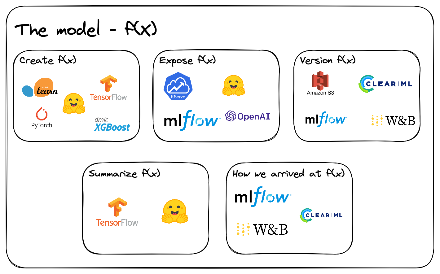
The model - \(f(X)\)

Let’s start with the most popular category - the model. Solving a problem from this category can be seen as a model-centric approach. Therefore, making it one of the most popular approaches as well. As we need a model to have an ML product.

Model creation

Before we can do anything, we need a model to use. Thankfully, tools such as sklearn, TensorFlow, PyTorch, etc., have made it possible to train a model with a few lines of code - model.fit(X, y).

This problem statement is what we see when being introduced to ML for the first time, and rightfully so.

However, this is only the start of even more questions. One natural question would be - How can we release a model, making it accessible to others?

Inference server

Meet one approach, an inference server. This approach often requires a separate server that handles model inference. Therefore, making it possible to access additional hardware like GPUs or TPUs if needed. As a result, an inference server is a standard solution.

However, typing up a new codebase only to make one model accessible can sound like a lot of work. Since an inference server is a common requirement, many solid solutions have popped up. For example, Huggingface offers a way to deploy transformer models within a few minutes, while OpenAI offers pre-trained models through an API. Then you have solutions like KServe, which makes it reasonably easy to deploy custom AI models on a Kubernetes cluster

But with our model deployed comes a new problem - What if I want to update my model to a new version?

Model Registry

Here is where the model registry comes in handy. In the same way we version code, will there be a need to version models at some point. Either because we found a new feature that could help or because the old pattern does not apply anymore - known as concept drift.

Therefore, we need to have some way of managing \(f_0(X), f_1(X), ..., f_n(X)\), and so on.

One simple way could be to store our models in a storage service like AWS S3. Such a solution can work if we have a few artifacts to handle. However, the complexity can quickly increase as we want the model to do more. For example, we could add pre-processing and post-processing, or we want to manage the runtime environment of the model. Using a more specialized model registry component for such a requirement would make sense. One such tool would be MLFlow.

But again, as we start to train new models regularly, new problems arise. For example, how will we know the differences between all our models?

Model Card

Here is where model cards come in. It summarizes what the model will do, how it was created, its limitations, some performance statistics, and more. Therefore, a model card summarizes \(f_n(X)\).

One tool that collects this information is model_card_toolkit. However, we will need to dive deeper into our model. So could we see how our model came to be?

Experiment tracking

Experiment tracking is one solution to such a problem. Providing a log of metrics as our model is trained, in addition, can all kinds of evaluation graphs be logged - as confusion matrices, and log which features contribute the most to our output. Therefore, answering how we arrived at \(f_n(X)\).

Some tools that answer this question are Weights & Biases, ClearML, and MLFlow.

Final thoughts on \(f(x)\)

The model category starts tackling problems from the model’s point of view. Answering a lot of the questions, such as how \(f(X)\) got created, when to use \(f(X)\), how to version \(f(X)\), and how we can expose \(f(X)\) to others.

However, we still have some huge questions to answer before we have a fully working ML system. Because, what is \(X\), and can \(X\) change how well our model performs? Such questions lead us to the next category.

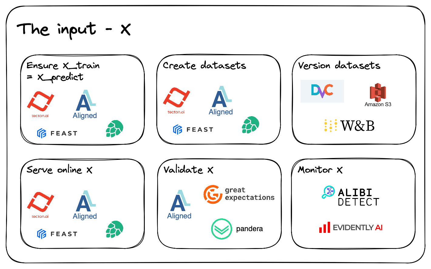
Input data - \(X\)

Introducing our second category - input data.

Someone jokingly said that ML practitioners use 99% of their time debugging and 1% writing code. However, there is some truth to this. It can be hard to debug ML products, and silent bugs can be one reason.

An example of a silent bug

To bring home this point, let’s look at a simple example. Let’s say we have a ride-sharing company that wants to predict the duration of a ride. So the ML researcher finds some data in a database containing the ride’s distance. Therefore, thinking this can be a good feature. And the performance metrics were outstanding when evaluating using the train, test, and validation set. Thus, you are convinced to release a new model version. However, we notice that our model performs way worse in production. How could this be?

We start debugging our data and notice that we estimate the distance when the ride starts but update our database with the actual duration when the ride has ended. Therefore, we have trained on the actual distance, but we predict an estimate. Thus, our model performance is worse in production. Such a bug is also known as data leakage.

Overwriting an estimate with the actual value may seem like a poor choice. Still, overwriting old data - known as slowly changing dimension 1 is common practice because it simplifies the queries in an application database. However, this makes making mistakes in ML products easier if we mutate data, as we may train a model on data from the future.

Data warehouse

One solution and a common component in business analytics is a data warehouse. A data warehouse is a single truth source for all analytical workloads. Making it optimal to compute aggregates on millions of records, and ML products can leverage this component.

Furthermore, since some data warehouses store a historical record of our data - potentially using slowly changing dimension 2, will it be possible to travel back in time. Therefore, it is possible to ask the question - what is \(X_{t}\) when \(t =\) the prediction time?

As an ML practitioners, this means we can create higher-quality datasets. Let’s use the ride-sharing example again. We may store our estimated distance value and the overwritten actual distance in a data warehouse but with a different timestamp. By correctly crafting our queries, we can select the values available at prediction time, training on the estimated value, which is the same data we predict on. Therefore, the new training set increases the performance of our model in production, leading to a more significant value gain for our end-users.

However, crafting such queries can be complex, and it is easy to make mistakes. Therefore, an ML researcher would like to think about something other than this - so what can we do about this?

Feature store

Here is where our feature store starts providing value.

A feature store acts as a highly specialized database for machine learning applications. One such use case will be how to generate data sets that would be valid at the time of prediction. Therefore, fulfilling the same needs as described as a data warehouse. However, the feature store abstracts away the complex queries and logic needed to provide such data. Also known as a Point-in-time correct join.

Therefore, creating a dataset where each row has the features that were available at their prediction time \(D = \{X_{0,0}, X_{1,0}, ..., X_{t,e} \}\) where \(t\) is the prediction time, and \(e\) is the entity to predict for.

Furthermore, we often want to engineer our features a bit, either by generating embedding features or something simpler as computing a ratio between two columns.

We could add some pre-processing into an artifact and store them with our model in a model register. However, some features require more computing. For example, features like mean distance over 20 minutes will be impossible in a serverless pre-processing method. But at the same time, we need to ensure that we use the same features in our training run and our online inference server. Otherwise, our prediction could be meaningless. This problem is also known as the training-serving skew.

Again, our second reason for a feature store. Ensure training and prediction features are the same \(X_{train} = X_{predict}\).

Lastly, there is one more reason to set up a feature store. We have covered how a feature store leverages a data warehouse to generate higher-quality datasets. However, loading inference features from a data warehouse often lead to long waiting times. This latency is because a data warehouse is optimized to analyze large amounts. Therefore, a data warehouse optimizes its hardware and disk usage for such use cases. However, this often leads to slower reads when we ask for individual rows of data.

As a result, a feature store fixes this limitation by changing the data storage based on the query type. Therefore, using a data warehouse for generating large datasets, but then using a key-value store for low latency inference data.

Some alternatives for feature stores are Feast, Tecton, Hopsworks, or my own solution Aligned.

Final thoughts on \(X\)

Ensuring data quality can be hard, as logical errors can easily creep in. Thankfully, a feature store can be a very useful component. Therefore, leveraging well-established data engineering practices abstracts away a lot of the complexity needed for ML products.

But still, there is one category left.

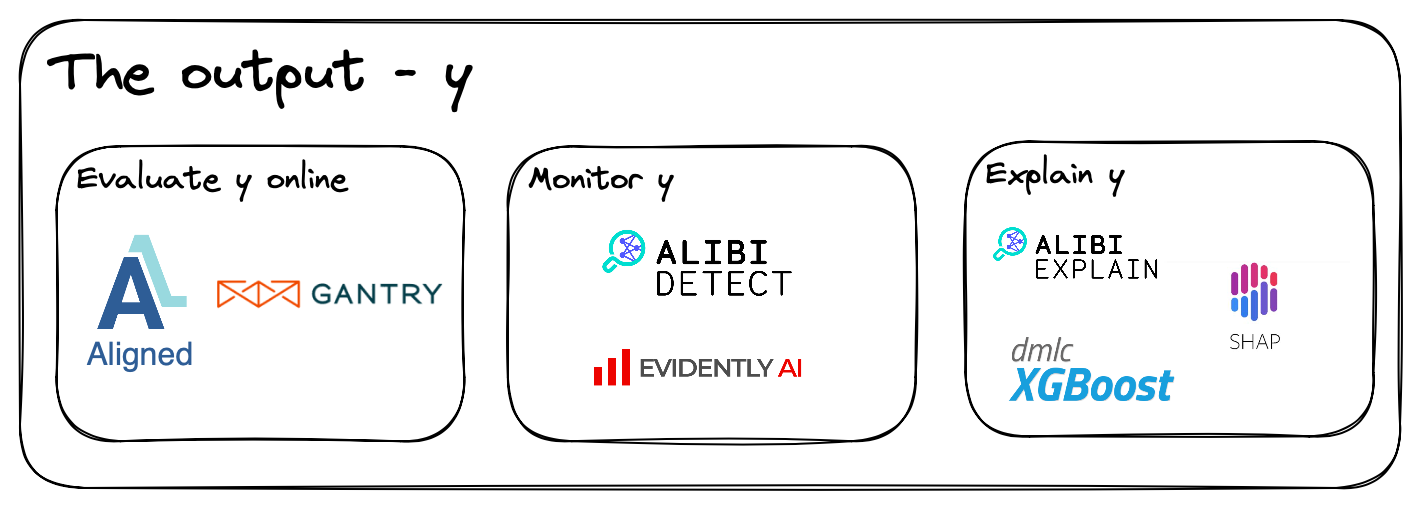
Output data - \(y\)

Lastly, we have the output data category. The output category could be in a joint data category with the input data. However, there are a few reasons for separating it into a separate category.

First of all, the leading players in the input data category do not provide a structured system to handle the output of our models.

Secondly, the output is the most critical artifact of them all, as this is what provides value for our end-users. All other components only exist to facilitate the creation of our \(y\) value.

However, more tooling is needed to make it easy to validate our online predictions.

Monitoring

From my experience have, the most popular solution been to set up a Prometheus and Grafana server for such use cases.

The Prometheus stack can work for simple needs. In the same way, S3 works well as a model registry when the artifact complexity is low.

However, ML-specific use cases can be hard to fulfill with such a stack. One such use case could be to view performance metrics based on sub-groups. This is very doable if we know the sub-group in advance, but it can lead to a low feedback loop if we want to check new sub-groups.

Evaluation store

Here we have the evaluation store component. A component that specializes in monitoring online performance for ML products. However, this can sometimes be down prioritised to setup, because we may think training evaluation is good enough. But this will not always be the case, because of data drift, and silent data bugs. Therefore, using an evaluation store uses ground truth to evaluate our online predictions \(y = \hat y\).

An evaluation store also enables viewing performance in sub-groups of interest, leading to a better understanding of our model’s limitations.

One tool here is Gantry, but other players are also starting to pop up.

However, we have still on question left - why did the model return such an output?

Explanations

Finally, the last component we will cover, explainers. Knowing why a model return an output can be very important for businesses. So important that businesses sometimes will release a less performant model that is explainable, rather than a more performant blackbox model. Therefore, an explainer answers why \(\hat y\).

Here can a lot of approaches be used. Such as analysing the inner workings of a model - checking a decision-tree’s splits, but this will not work for complex models as neural nets. Such models are black boxes, resulting in a need for different tooling. Thankfully, examples of useful tooling can be alibi explain, SHAP, and LIME.

Final thoughts on \(y\)

The road to a fully functional ML product is long and complicated. However, online prediction evaluation can be an afterthought for ML products, even though online predictions are their most important artifact. Therefore, potentially leading to solutions with more boilerplate code.

However, solutions like an evaluation store can help with this. Furthermore, tooling that explains our output can be crucial to provide the confidence and trust our ML products needs.

Wrap up

The amount of existing MLOps solutions is enormous, and this post only touches the tip of the iceberg. Concepts like drift detection and improving label data with active learning, to name a few. However, we can broadly categorize MLOps solutions into three groups. Managing the input \(X\), the model \(f(X)\), or the output \(y\).

Furthermore, managing our models has become extremely easy, as noted by Chip Huyen

…, with models being increasingly commoditized, model development is often the easier part.

However, managing our input data takes a lot of work, as it is easy to create faulty datasets. Furthermore, finding these data faults is hard. Thankfully, we have designed tools such as a feature store to reduce the number of potential flaws.

Lastly, managing our output data can quickly become an afterthought. Especially for companies that need more experience with ML products. As we quickly focus on the tooling making ML possible in the first place. Furthermore, the need for tooling to manage our model outputs can point to MLOps being immature.

However, many exciting MLOps solutions are trying to evolve the field further. One such tool is Aligned, removing the separation between \(X\) and \(y\), and unifying it more as a data category. So follow me and the Aligned repo for some exciting upcoming announcements!